> For the complete documentation index, see [llms.txt](https://techacademy.gitbook.io/data-science-wintersemester-24-25/llms.txt). Markdown versions of documentation pages are available by appending `.md` to page URLs; this page is available as [Markdown](https://techacademy.gitbook.io/data-science-wintersemester-24-25/exploratory-data-analysis-eda/data-visualization/crime-rate-over-time.md).
# Crime Rate Over Time
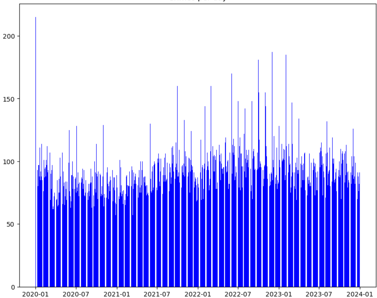
Let’s try some simple exploratory plots at first and look at the general trend of crime cases in general. Can we find interesting trends and/or relations of crimes cases?
* [ ] Plot the number of cases over time.
The result should look something like this:
Line plot
Barplot
How does your plot look like? A plot doesn’t have to be aesthetically pleasing, but has to convey your message without any further explanation. Another person should be able to get the quintessence of what you're trying to show by just seeing your plot. So let's add some more information.
* [ ] Add title and axis labels to your plot(s).
* [ ] Optional: Try different themes.
Does this plot help you explain what you wanted to explain? The plot seems to be very "noisy" which makes it hard to find a general trend. Let’s smooth the data to make trends better visible. Here we will plot a [rolling mean ](https://en.wikipedia.org/wiki/Moving_average)(a.k.a. moving average)
* [ ] Plot the rolling mean over 30 days over time. (*Hint: You can come up with your own implementation of the rolling mean or use already existing functions.)*
After this step, you should expect the plot to look something like this:
* [ ] Plot the rolling mean over 30 days grouped by the five most affected victim descents.
{% hint style="info" %}
🏴☠️: In order to get the number of crimes per month, use `group_by()` to group your data by month before summing over each day.
The `zoo` package has a function to calculate the rolling mean. You can find more about the rolling mean [here ](https://en.wikipedia.org/wiki/Moving_average)and more about the `zoo` package [here](https://www.rdocumentation.org/packages/zoo/versions/1.8-12).
{% endhint %}
{% hint style="info" %}
:snake:: To analyze time-series data, `resample()` is a powerful tool that adjusts the frequency of your data. Use it with datetime columns to group data into specific intervals (e.g., daily, monthly) and apply aggregation functions like `sum()`, `mean()`, or `size()`. Unlike `groupby()`, which requires explicit grouping columns, `resample()` works directly with time-based data, making it ideal for tasks like counting events per day or calculating averages over weeks. Combine it with methods like `rolling()` for smoothing trends and `unstack()` for pivoting multi-level indexes to prepare your data for visualization. Check the pandas documentation for more examples!
{% endhint %}
{% hint style="info" %}
The plots above are made with Python, if you're using R and your plots don't look identical don't worry!
{% endhint %}